Well, it might not be the fanciest thing in the world but it surely looks good when you try to visualize your data. You know me, I always graph whatever I do, otherwise I don’t get many ideas. I have to see what is going on, and perhaps are many people like me.

This time I’m gonna share a very simple and nice way to visualize the solution of a linear equation system with 3 unknowns and 3 equations.

Things you have to know:

1. An equation with 3 unknowns can be used to construct a plane. We will see how on further detail down.
2. If we have three independent equations and three unknowns, we have a unique solution. The three planes intersect at the same time in a single point
3. If two or more equations are the same (not independent), then their planes are the same. Thus there is no unique solution, because they would intersect in all points. Infinite number of solutions.
4. If two or more equations are proportional (not independent), then their planes are parallel. Thus there is no solution, because they would never intersect in any point. No solution exists.

Once we know this facts we can now move to the visualization of our data. Supose we are given a linear equation like this:

We can see that we have 4 parameters (a, b, c and d) and 3 unknown variables (x₁, x₂ and x₃). From here we can visualize a plane in 3D. How? Well, let’s rename our unknowns to each axis in 3D space:

x₁ = x
x₂ = y
x₃ = z

Which gives us:

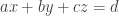
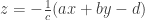
These unknown variables are gonna be used to graph every point with the given parameters. From here we clear for z to get:

Now check. We have only 2 independent unknown variables (x and y) and 4 given constant parameters (a, b, c and d). And these 6 values are our “inputs”.

Every time we use the 6 values we can get automatically the value of z through the formula above. What are they?

1. a, b and c are the parameters of the equation.
2. d is the value that the equation takes when evaluated with different variables for the unknowns… In simple words, when you know the parameters (a, b and c) and the values (x, y and z), you get d. In our case it’s viceversa: we know d but we should get z.
3. x and y are given parameters that we specify to our satisfaction. These two are the only input values that vary in the construction of our plane. Generally they are complete lists of numbers to evaluate, which in our case will be.

Ok. Ready for the action?

First, let’s create a random list of parameters a, b, c and d. In Matlab we will do it simply with:

p = rand(1,4);

This created 1 list with 4 random numbers and stored it in p.

Secondly, we create the list of values for x and y. As we want a plane, we first create a set of values in 2D (the two dimensions are x and y). In Matlab we easily do it with the function meshgrid, and in our example we will use values from -10 to 10:

[x,y] = meshgrid(-10:10);

The way it works is by creating two squared grids: one for x and the other for y. The x-grid will have values that increase horizontally (x-direction) from -10 to 10; while the y-grid has values that increase vertically (y-direction) from -10 to 10.

Please note that values of y increase from top to bottom.

x =

y =

With these grids it is easier to evaluate and create a plane. Just imagine they are superimposed one over the other. Then you start to evaluate for every point with the given input parameters:

The first element of x with the first element of y and the 4 inputs, then…
The second element of x with the second element of y and the 4 inputs, then…
The third element of x with the third element of y and the 4 inputs…

I think it’s pretty understandable by now, right?

This will evaluate 441 times because the grids are 21 elements large in every side. We take each value and put it in our equation. Remember our equation to get z?

With Matlab you can almost type it literally. Write it easily like:

z = -(1/p(3))*(p(1)*x + p(2)*y - p(4));

Note: Please have a look at it. The values of a, b, c and d were stored before in the vector p, we just call their corresponding indices, because:
p(1)=a
p(2)=b
p(3)=c
p(4)=d

Ta-daaaaaa! We got the complete set of values for z! Now we finally have the values of x, y and z that are needed to plot the plane.

In order to achieve this, we make use of the function surf in Matlab (it stands for ‘surface’). With this function we just put the list of values for each coordinate as:

surf(x, y, z);

Type that down and hit enter. Magic! There is your plane.

The complete code so far is like this:

p = rand(1,4);
[x,y] = meshgrid(-10:10);
z = -(1/p(3))*(p(1)*x + p(2)*y - p(4));
surf(x, y, z);

You must probably will see something like this (of course not the same because our parameters were generated randomly):

Not fancy enough, right? There are no lables for each axis and there is that awful grid on our plane.

But the party is not yet over! We are just warming up. So far we know how to plot a plane from a set of parameters and the x and y variables from our linear equation. Play with these basic concepts by now, generate again planes with random numbers or, even better, put some defined parameters from an equation and visualize it.

In the next post I’ll show you how to make it a function that we can use to plot any given equation as a plane, or 3 at the same time and their corresponding intersecting point, use fancy colors, get rid of unnecesary data and even show your equations and results in the command window… But that’s another story. See you in the next post!