The mystery is over! From the previous posts we have seen the way we can generate a random plane, and visualize 3 of them at the same time showing their intersecting point.

It might be enough for some simple visual purposes, but we are more ambitious than that and we want to get it fancier.

And that’s why I’m here! This final step would be to achieve a neat visualization of our three planes and even the equations involved. Let’s begin with what we have so far:

P = rand(3);
d = rand(3,1);
x = P\d;
hold on
drawPlane(P(1,:), d(1))
drawPlane(P(2,:), d(2))
drawPlane(P(3,:), d(3))
scatter3(x(1), x(2), x(3))

Where the function drawPlane was defined as:

function drawPlane(P, d)
[x, y] = meshgrid(-10:10);
z = -(1/P(3))*(P(1)*x + P(2)*y - d);
surf(x, y, z);

Color my face!

What can be improved from here? First thing that comes to my mind is the color of the planes. It is quite disturbing that the three have the same color-scaling and some times is not even possible to distinguish from each other because they might be too close.

So, I’ve thought on using 3 different colors to differentiate them: pink, light green and light blue. They are light because are not that aggressive to the eyes.

If you want to use a different set of colors, be my guest. My goal is to show how can we use them to improve our visualization.

Where do we change it? I presume it would be better by including the parameter of the color in every call to drawPlane. So, whenever we want to plot a plane, we immediately specify the color of it. This might look something like:

drawPlane(Parameters, Values, Color)

Where the parameter color will obviously specify the color of the plane.

Ok, open the file of the function drawPlane and analyze the code. The plotting happens when we call the function surf. We are giving the coordinates of every point of the plane. Let’s give the color. For that matter, we actually need 2 extra inputs: the name of the parameter to change and the new value.

By default, the surface plots created with surf have a color defined by their position in 3D. It means, the higher they are (large z), the “redder”. And the lower they are (small z), the “bluer”.

Because we want to have a uniform color throughout the plane we will say that the “face color” of the plane be of any given “color”. The line of surf will be modified to be now:

surf(x, y, z, 'FaceColor', color);

But I still see a very ugly thing in our planes: the grid. Yes, the planes have still those ugly meshes on top. I don’t like them, so I decided to disappear them with these two other parameters:

surf(x, y, z, 'edgecolor', 'none', 'FaceColor', color);

This, my friend, will make the edges “invisible”. No more mesh (nor mess).

Note: Remember to separate every input parameter with a comma. We don’t want to scramble our code with the simplest mistakes.

Now go to the first line. There you will also need to add an input named color. So, when you call this function you will have to specify the three things: parameters (P), values (d) and color. The first line will look like:

function drawPlane(P, d, color)

The parameter color (denoted in blue) must be literally the same (it’s case sensitive too) for both lines: in the definition of the function and in the line it’s going to be used, this case in surf. Otherwise, it will never find the variable and won’t work.

Save this file and return to the main one.

In the main file we are calling drawPlane with two parameters for each plane, but now we have to specify the color too.

In Matlab there are basically three ways to specify the color of a plot: long, short and vectorial. For a complete table of color references check Matlab’s online reference of the property ColorSpec.

We will use the vectorial way, because it allows us to manipulate the colors in every possible value, giving us the widest range.

For that purpose, we use a row-vector with 3 values of the RGB standard. That is 3 values between 0 and 1 that denote the color concentration of red, blue and green.

So, for instance, the vector [1, 0, 0] specifies a color with full concentration of red and none of green or blue. While the vector [0.5, 0, 0.8] say that we want half concetration of red, none of green, and 80% of blue.

As expected, the vector [1, 1, 1] is white and the vector [0, 0, 0] is black.

In our values of pink, light green and light blue for each plane, I have set it to:

drawPlane(P(1,:), d(1), [0.9 0.7 0.7]) % First plane (Pink)
drawPlane(P(2,:), d(2), [0.7 0.9 0.7]) % Second plane (Green)
drawPlane(P(3,:), d(3), [0.7 0.7 0.9]) % Third plane (Blue)

Check how the concentration of each color slightly changes in every plane.

Labeling the neighborhood

Great! Now, the final detail in the visualization of our planes is the labeling of the 3D space. Let’s identify every dimension as follows:

xlabel('x')
ylabel('y')
zlabel('z')

And we create a “sense” of depth if we add a grid to our background:

grid on

Boom! Execute this final beauty:

P = rand(3);
d = rand(3,1);
x = P\d;
hold on
drawPlane(P(1,:), d(1), [0.9 0.7 0.7]) % First plane (Pink)
drawPlane(P(2,:), d(2), [0.7 0.9 0.7]) % Second plane (Green)
drawPlane(P(3,:), d(3), [0.7 0.7 0.9]) % Third plane (Blue)
scatter3(x(1), x(2), x(3))
xlabel('x')
ylabel('y')
zlabel('z')
grid on

Great visualization! But I’m not yet satisfied. I also want to know what are the equations that were used in this system.

Display in Command Window

Well, we have that information stored in our matrix of parameters P, and the vector of values d.

In order to print the equations in the command window I use the function disp, where its input is a single string. This will display that string in a line in the Command Window. As we have many strings, even for a single equation line, I converted every value to a string using num2str and concatenated all strings to a larger one (look carefully, they are all stacked within the red brackets) to get a full equation. It works like this:

disp(string)

or if many strings are in a single line:

disp( [ string1, string2, ... , stringN ] )

I created a single loop that takes every value in the first column and matches it with x; every value of the second column and matched with y; and every value of the third column to be matched with z. In the right side of the equation, every equation is equal to their corresponding value of d.

For a better understanding check the code I used:

for i=1:3
    disp([' ', num2str(P(i,1)), 'x + ', num2str(P(i,2)), 'y + ',...
    num2str(P(i,3)), 'z = ', num2str(d(i))])
end

At the end of the first line inside the loop are three points. They are used to jump to the next line as if it was part of the original line, without breaking the command. It is very used to complete lines of code that are very large, like in this case.

That single loop prints the equation system taking the parameters from P, pairs them to their corresponding variable (x, y or z) and equals them to their values of d.

For a more “formal” presentation you can just add a title line for “Equation System” before printing it:

disp('Equation System:')

and a little space in the beginning of every equation. You can see it in the code above. Do you see the first element of the “stacked strings”? That’s right, a space.

And finally. It would be also nice to write down (not just show) where the intersection point lies. And that is as easy as the previous lines because we already have that point stored in our variable x, remember?

We will use the disp function again, so that we finally get:

P = rand(3);
d = rand(3,1);
x = P\d;
hold on
drawPlane(P(1,:), d(1), [0.9 0.7 0.7]) % First plane (Pink)
drawPlane(P(2,:), d(2), [0.7 0.9 0.7]) % Second plane (Green)
drawPlane(P(3,:), d(3), [0.7 0.7 0.9]) % Third plane (Blue)
scatter3(x(1), x(2), x(3))
xlabel('x')
ylabel('y')
zlabel('z')
grid on
% Display in Command Window
disp('Equation System:')
for i=1:3
    disp([' ', num2str(P(i,1)), 'x + ', num2str(P(i,2)), 'y + ',...
    num2str(P(i,3)), 'z = ', num2str(d(i))])
end
disp('The intersecting point (solution) lies on:')
disp([' x = ', num2str(x(1))])
disp([' y = ', num2str(x(2))])
disp([' z = ', num2str(x(3))])

We did it!

Those green lines are comments, so it doesn’t matter if you leave them or erase them. Doesn’t change the final result.

Execute those lines and check the result. In my case I stored this code in a file named test_solution_3_equations. You can, of course, name it as you want. So, when I execute mine, I get to see something like this:

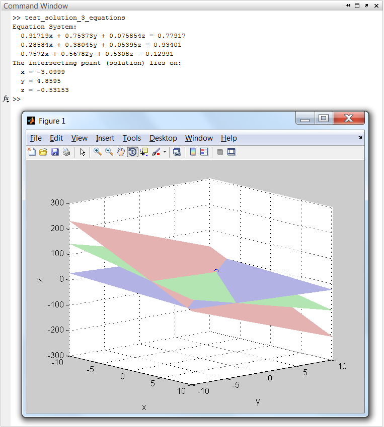
As the parameters are randomly generated, don’t expect to see the same equation system, nor the same planes.

So, first you see the execution of the file, followed by the equation system used to create the 3 planes intersecting.

Second, it shows the coordinates of the intersecting point of the planes.

Finally, in the new window that pops up, you can see the three planes with different colors and the point where they intersect. You can rotate the model with the “rotate 3D” tool (here you see it selected in the menu on the window).

Gorgeous!

Now it’s your turn to modify it and put as much as you want. You can even put your own given parameters, if they were already given, and solve instantly your equation system.

Improve it, maybe by adding an “error” routine telling you that two or even the three planes are parallel, therefore no solutions.

Or maybe there are 4 planes, maybe 5. What could happen? What would we use?

Is the Pseudoinverse ringing a bell?

Cool cool! Comments? Suggestions? Questions? Write down your fears!

See you around!