All right, I know I let you abandoned for a bit. But the last trip to Barcelona and the ongoing final exams in the University haven’t given me any chance to keep this. But I’m gonna take some minutes to finally write about the visualization of our planes.

In the last post we analyzed how a plane is constructed given the equation ax+by+cz = d. Then, given the parameters of this equation, I showed you how to generate its corresponding plane in Matlab.

Now I’m gonna keep this post short (sorry for the inconvenience), but here we are going to set 3 planes in a single visualization. In a third post, we’ll make all pretty and fancy.

Pedal to the metal! From last time I explained how to create and plot a random plane with the following lines in Matlab:

p = rand(1,4);
[x,y] = meshgrid(-10:10);
z = -(1/p(3))*(p(1)*x + p(2)*y - p(4));
surf(x, y, z);

But we want 3 Planes! No problem, my friend. And actually, adding them is extremely easy. However, we now realize that their plotting means to compute z 3 times. I know it’s not a problem for the computer, but the code might seem a bit “bulky” with those lines there.

So, a better idea is to create a function only for the plotting. Why? Because instead of writing this many times:

p = rand(1,4);
[x,y] = meshgrid(-10:10);
z = -(1/p(3))*(p(1)*x + p(2)*y - p(4));
surf(x, y, z);

We can just write something like:

drawPlane(input)

And it’s done! Sounds like a plan? If you’re with me in this, then let’s give it a try.

First, let’s define the inputs and outputs of our function:

If you remember from my post about how to use polyval, there are basically two inputs when we evaluate an equation: parameters (P) and variables (x,y) ; and one output: value (z).

The different values of z (outputs) draw the plane.

Our function takes the parameters and the list of values for x and y. But wait! In the first application we had, we have set the variables x and y to be between -10 and 10. Check the second line of the code above.

That’s right. So, for our goal (just a fancy visualization), we can bounder again our planes to be within those values every time. Now our inputs and outputs would look like:

Just because our variables will be set from -10 to 10 inside the function.

You may have a look at the first post. There, the equation of a single plane is defined as:

Or just changing the name of the variables:

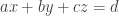
So, for three planes together it becomes the following set of linear equations:

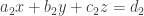
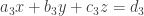
The first line corresponds to the first plane, the second line to the second plane, and the third… well, you know.

Represented with a Matrix multiplication, it turns out to be:

Which on broader detail is:

Do the multiplication yourself to confirm this.

But relax, our task doesn’t get more difficult, we just have to re-organize the way to represent our equations. They became easier! Why? Because instead of representing our parameters it with 3 separated vectors, we can do it with a single matrix.

Yes, that 3×3 matrix at the left side of the equation contains the parameters of the three planes. Where are our d’s? Those are in the vector at right side. This is, in fact, the easiest representation of the linear equations, although our inputs and outputs are now:

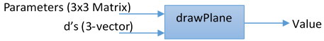
Thus, from the matrix representation above, we have to give the 3×3 Matrix P and the 3-column vector containing the d’s.

From the 3-column vector in the middle, we have fixed the values for x and y. With that, we get the values of z as our only output. Yei!

Function drawPlane

If you don’t know how to create a function in Matlab, this is your chance. It is going to be the easiest thing. To specify a function, the template is:

function output = functionName(input)

• function states that the file is a function. Write it like that, it must not be changed.
• output is the set of output values we want to get. We can put any name here.
• functionName is the name of the function. In our case will be drawPlane.
• input is the set of inputs we must give in. We have said that they will be 2: P and d.

Open a new file and the first line will express that it is a function:

function drawPlane(P, d)

It makes that file a function, so in any m-file that we execute it can be called as:

drawPlane(P, d)

Hey! Where is our output? No need to say that we don’t want the numerical values of, just the plotting. In case you want the outputs (z), just write:

function z = drawPlane(P, d)

But we are not going to use them for other than plotting, and that will be done already inside the function.

Now is time to specify the x and y as before:

[x, y] = meshgrid(-10:10);

Again, solving for z we get:

Which in Matlab is written as:

z = -(1/P(3))*(P(1)*x + P(2)*y - d);

We have now x, y and z (with 441 values each, so they are 21×21 matrices). Now we just plot the plane using surf:

surf(x,y,z)

Boom! Our function is 3 lines long, but when we call it in our main file, it will be a single line. Magic! So, the complete code for the function drawPlane so far is:

function drawPlane(P, d)
[x, y] = meshgrid(-10:10);
z = -(1/P(3))*(P(1)*x + P(2)*y - d);
surf(x, y, z);

Wanna test it? Save the file of the function with the name drawPlane (it must have the same name as your function) and go to the main M-file. In the main file (or even in the Command Window) clear everything and write:

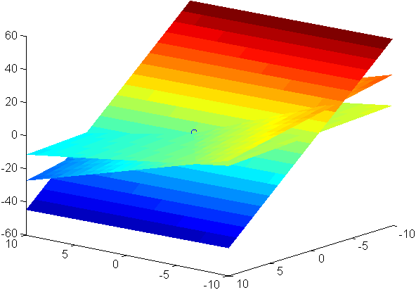
P = rand(3);
d = rand(3,1);
hold on
drawPlane(P(1,:), d(1))
drawPlane(P(2,:), d(2))
drawPlane(P(3,:), d(3))

Woah! Magic 3 planes in your screen. Don’t worry about the color and grids, we are going to make them disappear in the next post. For now we can plot 3 planes together and have created a function, so we are able to do it with a single line. Ahuaaa!

Oh yeah, if you’re not yet familiar with the notation of Matlab, P(1,:) means “in P, from the first row take all the elements”. When it is a single vector you do the same but with a single number, so d(1) means “from d take the first element”.

The instruction hold on before drawing the planes tells Matlab to hold the plots in your window. It will plot the planes in the same place. To deactivate it you ca use hold off.

If you don’t hold your plot, it will plot the first plane first, then will clear the window and draw the second, then clear it again for the third plane.

Finding the intersecting point

Now I would say that our application is ready to be prettier, but unfortunately it isn’t. Sure, we can now implement the “plane drawing” with a single line, but don’t forget that our goal is also to find the point where all the planes intersect.

But the funny part of this story is that we have to find the intersecting point. Why is it funny? Because it is one of the easiest things to do.

So, we have this equation:

P*x = d

Where:

• P is a 3×3 Matrix with the parameters of the equation.
• x = (x, y, z)^T is a vector that defines any point in 3D space.
• y is a vector with the values of each equation (the d’s).

What we want to find is the point where all the planes have the same value because they all intersect at this point. Simple Algebra and it’s easy-piece:

x = P^-1d

What? Yeah, that’s all. The point where all the planes intersect is given by that equation, which can be written in Matlab as:

x = P\y;

The backslash is used to get the inverse of a matrix, and we can do it because our Matrix is squared and invertible (although this last property is not 100% secured). It is equivalent to:

x = inv(P)*y;

But actually Matlab has a better computation with the backslash. Add that single line of code to our existent and you are almost done.

P = rand(3);
d = rand(3,1);
x = P\d;
hold on
drawPlane(P(1,:), d(1))
drawPlane(P(2,:), d(2))
drawPlane(P(3,:), d(3))

But why to get the intersection if we don’t visualize it as fancy as the planes? Let’s call scatter3!

We got our matrix P and vector d of the parameters. From there we got our vector x with the 3D coordinates of the intersecting point. And because Matlab is so nice with us, we can simply use the function scatter3 to show our 3D point in space:

scatter3(x(1), x(2), x(3))

Smooth as a princess’ cheek. The input parameters are simply the coordinates x, y and z that are contained in the vector x.

The final code so far has been:

P = rand(3);
d = rand(3,1);
x = P\d;
hold on
drawPlane(P(1,:), d(1))
drawPlane(P(2,:), d(2))
drawPlane(P(3,:), d(3))
scatter3(x(1), x(2), x(3))

with a function file drawPlane, whose code is:

function drawPlane(P, d)
[x, y] = meshgrid(-10:10);
z = -(1/P(3))*(P(1)*x + P(2)*y - d);
surf(x, y, z);

All right, it feels good to play with it, right? Execute your main file as many times as you want, in order to see the different plots it produces.

We finally plotted our three planes and their intersecting point. Now that we have it running we can carry on with the “upgrading” and make it fancy. That will be done in the next post. See you around!